Vibration Analysis Models for CNC Spindle Failure Prediction

A CNC spindle failure is the most expensive way to lose a week of production, and the choice of model, physics-based simulation, classical machine learning, or deep learning, decides whether a shop gets a two-week warning or a two-hour one. That gap is not a matter of taste. Bearings degrade over weeks, throwing off vibration signals that predictive models can catch long before a spindle seizes, but only if the model matches the signal it's reading and the conditions it has to read it under. Get that match wrong, and the warning window collapses to nothing.

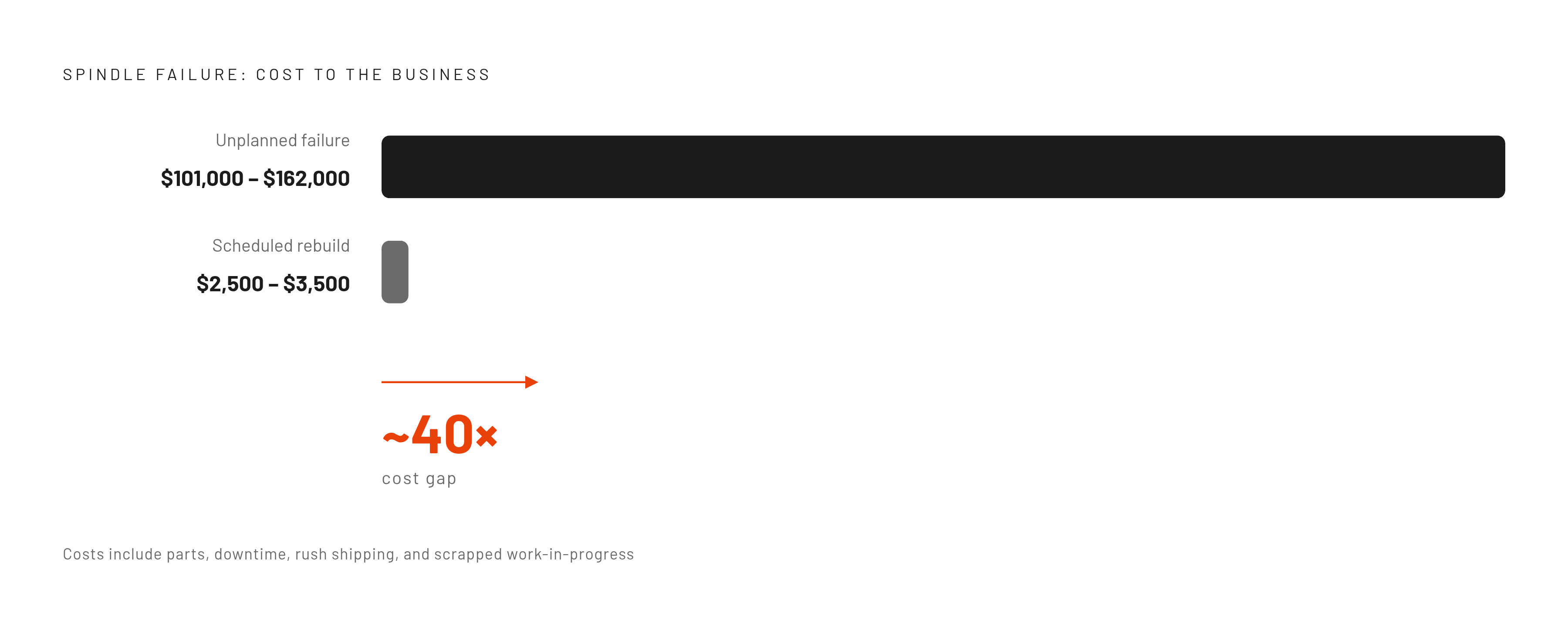
Spindles run at 15,000 to 30,000 RPM, and at that speed a minor bearing defect can turn into full seizure in under 200 operating hours. Fluke's survey work found that 61% of manufacturers polled had suffered unplanned downtime in the prior year. Replacement parts, two weeks of downtime, rush shipping, and scrapped work-in-progress add up fast: an unplanned failure runs somewhere between $101,000 and $162,000, against $2,500 to $3,500 for a scheduled rebuild caught early by a predictive system. That gap, roughly forty to one, is the whole argument for building these models correctly instead of picking whichever one sounds newest.

What a spindle's vibration signal contains and why raw data alone is insufficient

A spindle is an assembly: shaft, bearings, drive motor, preload mechanism, tool holder, and cutting tool. Each part throws its own vibration fingerprint into whatever the sensor picks up, and untangling those fingerprints is the whole job. It's harder than it sounds, because the fingerprints don't stay put.

Different failure modes leave different marks. Bearing wear starts as a progressive, impulsive signal that appears first in the high-frequency bands, long before anyone standing next to the machine could hear it. Imbalance and runout are periodic, tied to shaft rotation frequency, and they show up in an FFT as clean synchronous peaks. Chatter is trickier: a spindle can sound fine spinning under no load and still chatter badly once it's cutting, and a bearing that's lost stiffness may never produce the raceway noise a technician is trained to listen for. Misalignment and looseness live in the velocity signature, while acceleration data is where bearing health actually shows up, so a setup tracking only one of the two is monitoring half the spindle and calling it whole.

Bearing characteristic frequencies, the specific frequencies tied to a race or rolling-element defect, carry very little energy to start with. They get buried under noise and the much louder vibration of the machine's overall structure, and the signal never sits still long enough to make extraction easy, as spindle speeds swing from 5,000 to 30,000 RPM, cutting loads shift with material hardness, and coolant contamination and thermal drift add slow variation on top. None of this is stationary in the statistical sense. None of this is stationary in the statistical sense, so feeding raw vibration straight into a model without accounting for that produces noise wearing the costume of a prediction.

How signal processing transforms raw vibration into features a model can use

Three feature domains carry most of the load, and each catches something the others miss. Time-domain statistics like RMS and kurtosis are the simplest place to start: RMS tracks overall vibration energy, and kurtosis catches impulsive events, the earliest tell of localized bearing damage, because a healthy signal follows a roughly bell-shaped distribution while a damaged bearing throws sharp spikes that skew it. Frequency-domain analysis, mainly the FFT, shows what frequencies are present but throws away when they occurred, which makes it weak on its own for a signal that's localized in time. The old workaround was pairing FFT with envelope detection to isolate bearing characteristic frequencies directly.

Time-frequency methods fix that by preserving both when a transient happens and at what frequency, which matters for a signal that keeps shifting speed and load. A handful of these dominate the spindle literature, and picking one commits you to a downstream model, so the choice isn't cosmetic. The Short-Time Fourier Transform (STFT) uses a fixed window and runs cheap, trading some frequency resolution for speed, and it serves as the front end in the AWResNet study on rotation-error prediction. Wavelet Packet Transform (WPT) captures fault-related transients efficiently and pairs naturally with PCA to compress features before they reach a classical ML model. Variational Mode Decomposition (VMD) breaks a signal into intrinsic mode functions and has been paired with CNN-Transformer hybrids in the research literature, where the CNN picks up local features and the Transformer tracks dependencies across modes. Ensemble Empirical Mode Decomposition (EEMD) is built for nonstationary conditions specifically, decomposing signals into intrinsic mode functions from which informative features can be selected and passed to a downstream classifier.

Spectral kurtosis sits between the classical and the exotic. It adaptively finds the center frequency and bandwidth where impulsive content concentrates, builds a bandpass filter around that, and applies a Hilbert transform to pull out the envelope spectrum, giving a precise read on fault frequencies without any deep learning involved. Whatever feature extraction gets picked here decides what model can come next. That's the hinge the rest of this piece turns on.

Physics-based and classical ML models

Physics-based models start from the mechanics of the spindle itself, and they're the right call whenever geometry and material data are known and interpretability isn't optional. Skip this route the moment a spindle's maintenance history gets messy or its wear state drifts outside what the model was built around, because that's exactly where physics-based methods stop generalizing. A lumped mass model captures the nonlinear, nonsmooth restoring force generated inside a bearing along with the spindle's broader dynamics, often modeled across 18 degrees of freedom. Stability Lobe Diagrams, built from Frequency Response Function data, map which combinations of spindle speed and depth of cut are stable versus which will chatter, and they stay useful for process planning before a part ever gets cut. A framework published in September 2026 in IJIDeM combined Timoshenko beam theory with Random Forest Regression to predict tool-tip FRF on Al6061 alloy, hitting an R² of 0.999, evidence that machine learning can stand in as a cheap surrogate for expensive finite-element simulation.

Classical ML fills a different gap, and it earns its keep specifically where labeled data is thin and fault classes are already known. A pipeline combining PCA and Wavelet Packet Decomposition feeding into an LSTM classifier reached 97% accuracy distinguishing between bearing states. Spectral kurtosis paired with a Least-Squares SVM works well when fault classes are already well understood: the envelope spectrum from the Hilbert transform pins fault frequencies precisely, and the whole pipeline is light enough to run without much compute. Random Forest, used as an FRF surrogate, beats simple polynomial regression, especially at higher frequencies, another case of classical ML doing production work that used to require full simulation.

What ties both approaches together is a dependence on labeled fault data, stable-ish operating conditions, and hand-built features. Pulling out any one of those three degrades the pipeline. Deep learning entered the picture once conditions stopped being stable and labels stopped being available.

LSTM and bi-LSTM for remaining useful life estimation

Bearing degradation unfolds over time, and a single snapshot of vibration features can't tell early-stage wear apart from ordinary day-to-day variation. Estimating remaining useful life needs a model that learns the trajectory.

One IIoT framework built exactly that: an accelerated run-to-failure testbed generated spindle degradation time-series data, with Neighborhood Component Analysis selecting the most useful features before training. A standalone LSTM produced an RMSE of 40.01 time-steps and A20-index scores of 97.30% and 92.57% across two test datasets, and among the architectures tested, it came out the most balanced and the most consistent across conditions. A hybrid LSTM plus bi-LSTM pushed accuracy further on one dataset (RMSE of 31.65 time-steps, A20-index of 99.72%) but dropped on the second. That drop is the overfitting risk that comes standard with more complex architectures trained on limited data, and it's the reason a standalone LSTM, not the hybrid, should be the default unless the accuracy gain on one specific machine is worth the added validation burden. The framework ran on a MATLAB-powered ThingSpeak IoT platform, with real-time data acquisition, cloud-side analytics, a remote dashboard, and automated failure alerts.

Hybrid ensemble approaches that combine LSTM-based temporal modeling with gradient boosting have appeared in the literature as a way to fuse features across domains, with reported accuracy and lead-time gains over simple threshold-based vibration monitoring. A pure LSTM tends to generalize better across different machines. Hybrid architectures may squeeze out more accuracy on a single machine's data but demand careful validation before anyone trusts them somewhere else, and most write-ups skip that validation step.

CNN and hybrid architectures that treat vibration as an image classification problem

Convert a 1D vibration signal into a 2D image, using STFT, VMD, or GAF encoding, and a CNN can learn the spatial fault pattern directly, no hand-crafted features required. That single move is the core of a growing set of hybrid architectures, because it removes the feature-engineering bottleneck that limits classical ML.

AWResNet pairs an Adaptive Weighted ResNet with STFT front-end processing across multiple sensor channels. The architecture builds attention-weighting units on top of residual connections, and stacking these blocks lets the model adaptively weight which sensor channels matter most while quieting the redundant ones. Visualizing those learned weights shows the model picking up channel importance that actually maps onto something interpretable, which chips away at the usual black-box complaint leveled at CNNs, at least partially. On spindle rotation-error prediction, AWResNet outperformed the other deep learning models it was tested against.

The VMD-CNN-Transformer hybrid splits the labor differently. VMD decomposes bearing vibration into several intrinsic mode functions, the CNN handles fine local patterns within each, and multi-head self-attention in the Transformer layer picks up global dependencies across modes. That matters when a fault shows symptoms across several frequency bands at once instead of sitting in one clean band.

A third pipeline, EEMD plus GAF plus CNN, is built for variable-speed conditions where stationarity can't be assumed. EEMD handles the nonstationary signal, correlation-coefficient selection trims the intrinsic mode function count to the useful ones, GAF encoding turns the result into a 2D image that preserves temporal correlation, and the CNN classifies fault state from that image. It's the heaviest of the three pipelines, and it's also the one built for the messy, speed-varying conditions an actual shop floor produces, rather than the clean, fixed-speed conditions a lab bench produces.

Choosing among signal processing approaches, classical ML, and deep learning for a given deployment

No model here wins across the board, and anyone pitching one that way is skipping the part where the operating environment decides the answer. A few things settle most of it.

Start with how well the fault classes are already known. Known failure modes, bearing outer race defects, imbalance, misalignment, are well served by spectral kurtosis plus SVM or a PCA-WPD pipeline, and reaching for deep learning here is overkill more often than not. Unknown or compound failure modes, where several things go wrong at once, favor deep learning instead, because that's where hand-built features stop capturing what's actually happening. Data availability draws its own line: classical ML and physics-based models can work with limited labeled data, while LSTM and CNN architectures need run-to-failure histories or accelerated testbed data to train against, data that isn't always sitting around waiting to be used.

Operating condition variability matters just as much. A fixed-speed, stable-load spindle can usually get by on FFT plus envelope analysis, or a classical ML pipeline, and building anything heavier for that case wastes engineering time better spent elsewhere. A spindle running variable speeds and variable loads needs time-frequency methods like VMD or EEMD, or a sequence model like LSTM, because the stationary assumption simply doesn't hold there. The output you actually need matters too: fault classification points toward CNN or SVM, while a remaining-useful-life estimate points toward temporal models like LSTM or LSTM-GBM.

Interpretability cuts a different way. Regulatory environments or quality audits favor physics-based Stability Lobe Diagrams and spectral kurtosis pipelines precisely because they can be explained line by line to an auditor, while floor monitoring can tolerate a degree of model opacity that a regulatory audit cannot. Compute context closes the loop: edge-constrained sensors favor lightweight classical ML, while cloud-connected IIoT platforms like ThingSpeak can run full LSTM or CNN inference with real-time dashboards and alerting built in.

Hybrid architectures like LSTM-GBM or VMD-CNN-Transformer generally beat single-method approaches on raw accuracy, but they carry more complexity and heavier data requirements, and that trade only pays off when the accuracy gain justifies the engineering cost of building and maintaining the thing. The 68-hour lead time reported for LSTM-GBM, and the broader 4 to 8 week window vibration analysis can realistically offer, are the numbers a maintenance team actually plans around. A model that scores well on a test set but misses that window hasn't solved the problem the spindle actually has.